Neural HMM Model for POS Tagging
in Machine_learning / Machine Learning on Nlp
Let us define the HMM model for assigning POS tags. Let’s assume that we observe the words in a sentence. The emission of words is governed by a hidden Markov process that explains the transition between PSO tags. This HMM model can be described with the following graph
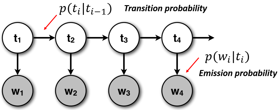
where \(t_i\) is a tag at position \(i\) and \(w_i\) is a word at position \(i\).
The joint probability of words and tags can be factorized in the following way \[\begin{aligned} p(w_1,...,w_N,t_1,...,t_N) &= \prod_{i=1}^N p(w_i \vert t_i)p(t_i \vert t_{i-1}) \\ &= \prod_{i=1}^N \frac{p(t_i \vert w_i)p(w_i)}{p(t_i)} p(t_i \vert t_{i-1}) \\ &= \prod_{k=1}^N p(w_k) \prod_{i=1}^N \frac{p(t_i \vert w_i)}{p(t_i)} p(t_i \vert t_{i-1}) \end{aligned}\]
assume \(p(t_1 \vert t_0) = p(t_1)\) for the simplicity of notation. We took the probability of each word in the sequence out of the product because, as we will see later, we can ignore them during the optimization.
Making your calculations with probabilities directly is bad for two reasons:
- When multiplying a lot of probabilities, you will face the problem of floating point underflow
- Multiplication operation is slow. You will have much higher performance if you calculate log of probability and then add log probabilities together
Viterbi Algorithm
In the problem of POS tagging, we want to maximize the joint probability of assigning the tags to the input words. Thus, the problem can be solved with a maximization objective \[\hat{t_1},..,\hat{t_N} = \underset{t_1,..,t_N}{argmax} \left( \sum_{i=1}^N \log p(t_i \vert w_i) - \log p(t_i) + \log p(t_i \vert t_{i-1}) \right)\]
The additive term \(\sum_{k=1}^N \log p(w_k)\) does not influence the result of summation, and therefore can be omitted.
Now, we want to solve this problem optimally, meaning given the same input, and the same probability distributions, you find the best possible answer. This can be done using the Viterbi algorithm.
Assume that you have an HMM where the hidden states are \(s={s_1, s_2, s_3}\), and the possible values of the observed variable \(c={c_1,c_2,c_3,c_4,c_5,c_6,c_7}\). Given the observed sequence \(\mathbf{y}=[c_1,c_3,c_4,c_6]\), the Viterbi algorithm will tries to estimate the most likely transitions \(\mathbf{z}=[z_1,z_2,z_3,z_4], z_i\in c\), and store the path of the best possible sequence at every step.
Define \[\delta_t(j) = \underset{z_1,..,z_{t-1}}{max}{p(\mathbf{z}_{1:t-1}, z_t=j \vert y_{1:t})}\]
This is the probability of ending up in state j at time t, given that we take the most probable path. The key insight is that the most probable path to state j at time t must consist of the most probable path to some other state \(i\) at time \(t − 1\), followed by a transition from \(i\) to \(j\). Hence \[\delta_t(j) = \underset{i}{max}\ \delta_t(i) p(s_j \vert s_i) p(y_t \vert s_j)\]
We also keep track of the most likely previous state, for each possible state that we end up in: \[a_t(j) = \underset{i}{argmax}\ \delta_t(i) p(s_j \vert s_i) p(y_t \vert s_j)\]
That is, \(a_t(j)\) tells us the most likely previous state on the most probable path to \(z_t = s_j\). We initialize by setting \[\delta_1(j) = \pi_j p(y_1 \vert z_j)\]
where \(\pi_j\) is a prior probability of a state. If we do not have this available, we can use the best unbiased guess - uniform distribution. The Viterbi algorithm will create two tables, that will store the following values
Probabilities:
| State | t=1, \(y_1=c_1\) | t=2 \(y_2=c_3\) | t=3 \(y_3=c_4\) | t=4 \(y_4=c_6\) |
|---|---|---|---|---|
| \(s_1\) | 0.5 | 0.045 | 0.0 | 0.0 |
| \(s_2\) | 0.0 | 0.07 | 0.0441 | 0.0 |
| \(s_3\) | 0.0 | 0.0 | 0.0007 | 0.0022 |
Best previous state:
| State | t=1, \(y_1=c_1\) | t=2 \(y_2=c_3\) | t=3 \(y_3=c_4\) | t=4 \(y_4=c_6\) |
|---|---|---|---|---|
| \(s_1\) | - | 1 | 1 | 1 |
| \(s_2\) | - | 1 | 2 | 2 |
| \(s_3\) | - | - | 2 | 2 |
The solution can be visualized as follows
 Source: Machine Learning Probabilistic Perspective, Chapter 17.4.4
For more thorough overview of Viterbi algorithm, refer here
Estimating Word Tags
The Viterbi algorithm requires you to estimate probabilities of tags for words \(p(t \vert w)\). We suggest using a time-tested convolutional architecture for sequence classification, inspired by the paper A Unified Architecture for Natural Language Processing: Deep Neural Networks with Multitask Learning (Check References for more reading).
Method
The main problem with tag classification for words is that the length of words varies, and it is unclear which features are useful for POS classification. It the best practice of Deep Learning, we create a model that learns useful features on its own.
The idea of the classification model is the following.
- Represent a word as a sequence of characters
- Use a projection layer to embed each character in a sequence. Each character will be represented with a real vector \(v_c \in \mathcal{R}^d\), where \(d\) is the embedding vector length.
- Apply convolutional layer with a non-linearity to extract higher level features from letters. The convolutional window has a size (\(d\), \(d_{win}\)), where \(d\) is the embedding length, and \(d_{win}\) is the width of the convolutional window. Typically set to 3 or 5. Pass over the letter embeddings without with stride of 1. The number of filters should be equal to \(h_{hidden}\).
- After applying the convolutional layer, you will have a series of embeddings of size \(h_{hidden}\). At this step, we want to flatten the input to make it independent of the sequence length. Do this by performing maxpool operation over the sequence length. As a result, you will get a word embedding of fixed size. During training, You are going to enforce morphological features captured in this embedding.
- Apply a regular NN layer to the word embedding and use softmax to estimate a probability distribution over tags.
 Source: Named Entity Recognition with Bidirectional LSTM-CNNs
Implementation
Unfortunately, it is not efficient to model sequences of variable length. For this reason, we are going to fix the length of a word to a maximal sequence length the same way as when using RNN. Therefore, the placeholder for the word is defined as
input = tf.placeholder(shape=(None, max_word_len), dtype=tf.int32)
The input contains integer identifiers for characters. The projection layer is similar for any word embeddings
tf.nn.embedding_lookup(embedding_matrix, input)
# produces tensor with shape (None, max_word_len, embedding_size)
Most convolutional layers accept a 4d tensor as an input, so look into tf.expand_dims to adapt the output of your projection layer.
Convolutional layer can be created with tf.layers.conv2d. You will need to specify the input, kernel shape, and the number of filters. The number of filters should be equal to \(h_{hidden}\). The output shape of the convolutional layer should be (None, max_word_len, 1, h_hidden).
Now you need to apply maxpool operation. The output of maxpool should be of shape (None, h_hidden). use reshape before maxpool if necessary.
The final NN layer should have the number of output units equal to the number of POS tags.
With this method, after training for two epochs, we have obtained the following per-word-accuracy score
loss 0.2043, acc 0.9323
and the following confusion matrix 
Read more about confusion matrix here.
Dataset Description
You are going to use a modified conll2000 dataset to train your HMM tagger. The dataset has the following format
word1_s1 pos_tag1_s1
word2_s1 pos_tag2_s1

word1_s2 pos_tag1_s2
word2_s2 pos_tag2_s2
word3_s2 pos_tag3_s2

word1_s3 pos_tag1_s3
...
wordK_s3 pos_tagK_s3

...
...
...
wordM_sN pos_tagM_sN
Where s* corresponds to different sentences. Every line contains an entry for a single word. Sentences are separated from each other by an empty line.
Assignment Details
The assignment is split into two parts: mandatory and optional. You can receive one point for each.
Mandatory Part
In the mandatory part, you need to implement the Viterbi algorithm. Use train_pos.txt to estimate transition probabilities \(p(t_i \vert t_{i-1})\) between different parts of speech tags. You can also estimate prior probabilities of tags \(p(t)\) from this file.
You are also provided with a file that maps a word into a distribution over POS tags. This file is stored in TSV format (we do not use CSV because some of the tags contain commas themselves). Each cell is a logit (log probability with offset) of the corresponding tag, i.e. \(\log p(t_i \vert w_i) + C\). The absolute value of a logit is not important, it is important how logits rank relative to each other. Higher logit value means higher probability.
The quality of your implementation is measured with the help of test set. Your final goal is:
- implement the Viterbi algorithm
- estimate the best tag assignment for each sentence in the test set
- report per-word accuracy on the test set in the output of your program
Optional Bonus Part
In the mandatory part, you use precomputed probabilities of word tags \(\log p(t_i \vert w_i)\). In the bonus part, you need to implement your own algorithm that estimates the probability of tags for words. You can use the method explained in section Estimating Word Tags. If you decide to implement your own algorithm, make sure that it works better than the suggested baseline, and provide a human-readable explanation of your method.
Report per-word tagging accuracy in the output of your program.
References
- A Unified Architecture for Natural Language Processing: Deep Neural Networks with Multitask Learning
- Convolutional Neural Networks for Sentence Classification
- Improving Word Embeddings with Convolutional Feature Learning and Subword Information
- A Primer on Neural Network Models for Natural Language Processing
- HMM for POS tagging